Convulations to CNN

We will study convolution, which is a popular array operation that is used in various forms in signal processing, digital recording, image processing, video processing, and computer vision. In these application areas, convolution is often performed as a filter that transforms signals and pixels into more desirable values.

In high-performance computing, the convolution pattern is often referred to as stencil computation. Convolution typically involves a significant number of arithmetic operations on each data element. Each output data element can be calculated independently of each other, a desirable trait for parallel computing. On the other hand, there is substantial level of input data sharing among output data elements with somewhat challenging boundary conditions. This makes convolution an important use case of sophisticated tiling methods and input data staging methods.

Convolution is an array operation where each output data element is a weighted sum of a collection of neighboring input elements. The weights used in the weighted sum calculation are defined by an input mask array, commonly referred to as the convolution kernel. We will refer to these mask arrays as convolution masks. The same convolution mask is typically used for all elements of the array

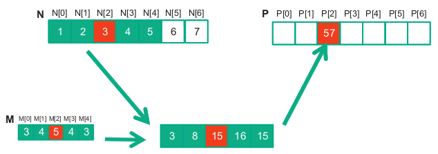
Below is shown a convolution example for 1D data where a 5-element convolution mask array M is applied to a 7-element input array N.

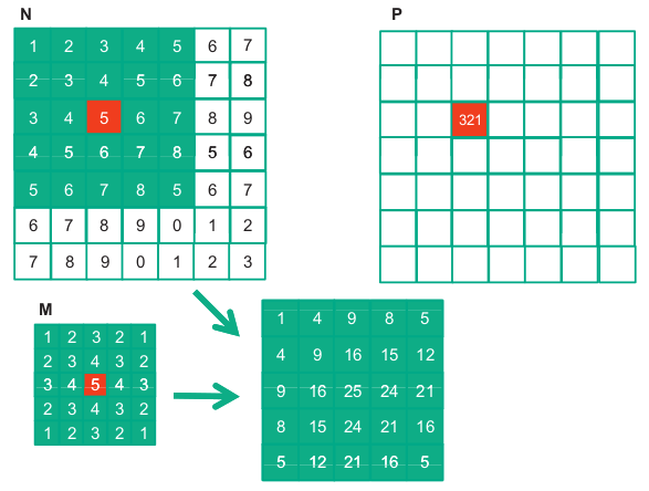
For image processing and computer vision, input data are typically two-dimensional arrays, with pixels in an x-y space. Image convolutions are therefore 2D convolutions. The mask does not have to be a square array.

1. From 1D to 2D convolution

You know 1D convolution:

• Input: 1D array (e.g., [x0, x1, x2, ...])
• Kernel: small 1D array (e.g., [w0, w1, w2])
• Operation: slide the kernel and take weighted sums.

For images, the input is 2D (height × width), so:

• Input: matrix of pixels, shape H × W
• Kernel: small matrix, e.g. 3 × 3 or 5 × 5
• Operation: place the kernel over each 3 × 3 patch of the image, multiply element wise, sum → one output pixel.

This is just the same idea you already know, but:

• Array → 2D array (matrix).
• Neighboring “elements” → neighboring pixels in 2D.

2. Multiple channels (e.g., RGB)

Real images are not just 2D, they often have channels:

• Shape: H × W × C (e.g., C = 3 for R, G, B).
• Then a kernel also has depth C:
  • Shape: kH × kW × C.

Convolution step:

• For one position, you take a small cube: kH × kW × C.
• Multiply elementwise with the kernel kH × kW × C.
• Sum all values → 1 number (one output channel value at that location).

So conceptually: 3D convolution over space + channels, but still just “weighted sum of neighbors”.

3. Filters (kernels) and feature maps

In CNNs, you don’t use just one kernel; you use many:

• Suppose you use F different kernels.
• Each kernel has shape kH × kW × C_in.
• Each kernel produces one output channel, called a feature map.

So if the input shape is:

• H × W × C_in,
  and you use F kernels, the output shape becomes:

• H_out × W_out × F.

Each of those F output channels captures a different kind of pattern:

• One kernel may learn to detect edges, another corners, another textures, etc.

Think:
“A CNN layer = apply many different convolutions (filters) over the input.”

4. Stride and padding

Two more array-related details:

• Stride: how far you move the kernel each step.

  • Stride 1: move 1 pixel at a time → dense output.
  • Stride 2: skip every other pixel → smaller output.

• Padding: add zeros around the border of the image.

  • Without padding, output gets smaller.
  • With padding, you can keep the same height/width.

Mathematically, it’s still just sliding windows and dot products, but with control over:

• How far you slide (stride).
• Whether you lose border information (padding).

5. Nonlinearity: adding activation functions

So far it’s all linear: weighted sums. A CNN layer adds nonlinearity:

• After convolution, apply an activation function elementwise
  (e.g., ReLU(x) = max(0, x)).

So a single conv layer is:

1. Convolution (linear weighted sums).
2. Activation (nonlinear).

This combination lets CNNs learn complex, non-linear mappings.

6. Stacking layers → deep feature hierarchies

A full CNN is just many layers of:

• Convolution → activation (→ sometimes pooling).

Intuition:

• Early layers: detect simple things (edges, blobs).
• Middle layers: combine them into textures, shapes.
• Later layers: combine shapes into object parts and objects.

All of this is still built from the same primitive you understand:
“take local neighborhoods and compute weighted sums.”

7. Connection to fully connected (dense) layers

A fully connected layer is also just weighted sums:

• Input: 1D vector.
• Output unit = sum of (weight × input) + bias.

Difference:

• Dense layer: every output unit uses all input elements.
• Conv layer: each output unit uses only a local neighborhood (sparse connectivity) and shares weights across positions.

So you can see CNNs as:

• A clever way to use your convolution operation to get:
  • Locality (nearby pixels matter more).
  • Weight sharing (same kernel across all positions).
  • Fewer parameters than a dense layer on full images.

Conclusion: From Simple Operation to Powerful Networks

If you understand convolution as:

“At each position, take neighbors and compute a weighted sum with a kernel,”

then you’re already standing on the core idea behind CNNs.

CNNs take that simple building block and:

• Extend it from 1D arrays to 2D/3D tensors.
• Apply many different kernels in parallel to produce rich feature maps.
• Add nonlinearities to escape pure linearity.
• Stack many such layers so that each stage “sees” more abstract structure.

The magic of CNNs isn’t a new kind of math—it’s the composition of many small, local, convolution operations into a deep architecture that can learn powerful visual representations.